R'Omic: high-dimensional data manipulation • romic

Core data structures

R ’Omic revolves around data structures for representing high-dimensional data. The data model can most easily be seen from the triple_omic object which represents features, samples, and measurements with a compact relational schema.

features - one row per feature (e.g., gene, transcript, metabolite)
samples - one row per sample
measurements - one row per observation (of a single feature in a single sample)

The relationships among variables in these tables are tracked using a design table which identifies the feature, and sample primary keys which uniquely define a feature or sample. This table also tracks the variables associated with features, samples, and measurements so these tables can be joined and re-arranged. This feature is taken advantage of to aggregate the features, samples, and measurements into a single tidy_omic table.

Example Data

To demonstrate romic’s functionality, this vignette will focus on analysis of the Brauer et al. 2008 yeast gene expression experiment. In this experiment, the impact of a yeasts’ nutrient environment and growth rate on gene expression was explored using 2-color microarrays. There are 36 samples, organized in a full-factorial design (all x all levels), which differ in terms of which nutrient limits growth and how fast the culture is growing.

Limiting nutrient: growth is limited with reduced levels of Nitrogen, Phosphorous, Leucine, Uracil, Glucose or Sulfur.
Dilution rate: 0.05-0.3 hrs^-1, is the rate that the culture is diluted and fresh media is supplied. This sets up a chemostationary condition where growth rate is entrained to the dilution rate.

Dataset Creation

library(dplyr)
library(romic)

A tidy_omic dataset can be loaded by passing a data table and specifying which variables are unique to features, samples and measurements

tidy_brauer <- create_tidy_omic(
  df = brauer_2008,
  feature_pk = "name",
  feature_vars = c("systematic_name", "BP", "MF"),
  sample_pk = "sample",
  sample_vars = c("nutrient", "DR")
)

## 1 measurement variables were defined as the
## left overs from the specified feature and sample varaibles:
## expression

A triple_omic dataset can be loaded by providing a features, samples, and measurements tables and specifying which variarbles are the features’ and measurements’ primary keys.

triple_brauer <- create_triple_omic(
  measurement_df = brauer_2008 %>% select(name, sample, expression),
  feature_df = brauer_2008 %>% select(name:systematic_name) %>% distinct(),
  sample_df = brauer_2008 %>% select(sample:DR) %>% distinct(),
  feature_pk = "name",
  sample_pk = "sample"
)

Generally, we wouldn’t maintain both a triple and tidy omic version of a dataset but rather convert back and forth between these representation based on the needs of the analysis. To convert between these classes we can use:

# convert back and forth between tidy and triple representations
triple_brauer <- tidy_to_triple(tidy_brauer)
tidy_brauer <- triple_to_tidy(triple_brauer)

Data Manipulation

Most functions actually don’t care whether you provide a tidy or triple representation of your dataset. These functions take a T*Omic object (i.e., tidy or triple omic), and apply an operation and return whichever class was provided. We can see this by filtering a triple_omic.

filtered_brauer <- brauer_2008_triple %>%
  filter_tomic(
    filter_type = "category",
    filter_table = "features",
    filter_variable = "BP",
    filter_value = c("protein biosynthesis", "rRNA processing", "response to stress")
  ) %>%
  filter_tomic(
    filter_type = "range",
    filter_table = "samples",
    filter_variable = "DR",
    filter_value = c(0.05, 0.2)
  )

We could also modify a table directly and then update it in the tomic object. For this workflow, update_tomic is used so the design can keep up with any fields that have changed.

updated_features <- brauer_2008_triple$features %>%
  dplyr::filter(BP == "biological process unknown") %>%
  dplyr::mutate(chromosome = purrr::map_int(systematic_name, function(x) {
    which(LETTERS == stringr::str_match(x, "Y([A-Z])")[2])
  }))

updated_tomic <- update_tomic(
  brauer_2008_triple,
  updated_features
)

Visualisation

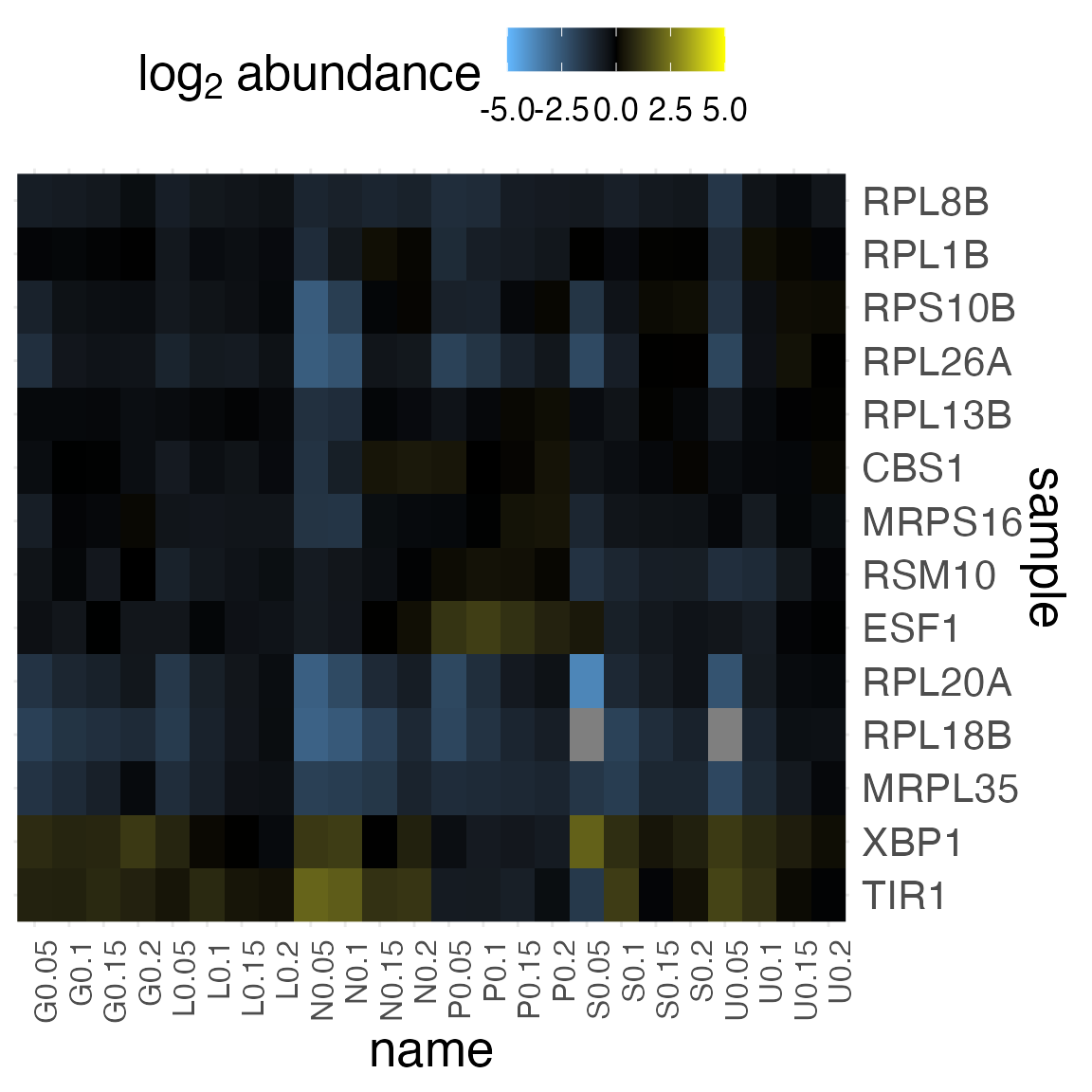
Romic includes a few versatile ggplot2-based plotting functions which can show a complete set of measurements, as a heatmap, or univariate/bivariate slices of features, samples or measurements.

plot_heatmap(
  filtered_brauer,
  value_var = "expression",
  change_threshold = 5,
  cluster_dim = "rows",
  plot_type = "grob"
)

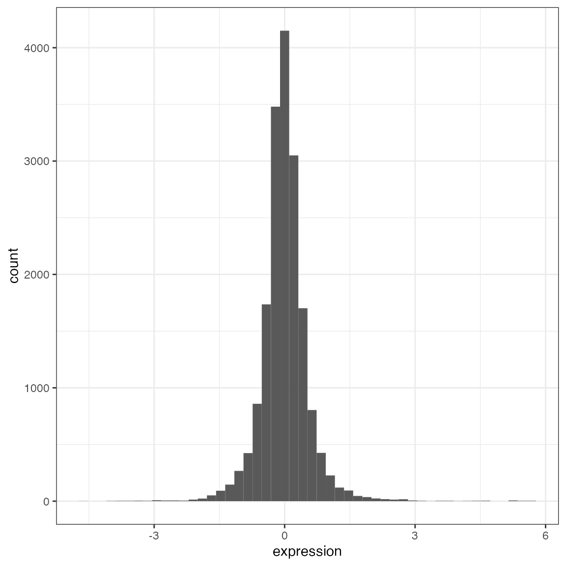
centered_tidy <- tidy_brauer %>%
  center_tomic()

plot_univariate(
  centered_tidy$data,
  x_var = "expression"
)

Interactive Visualisation

Romic maintains a valid data model when various operations are performed, and includes visualization which flexibly allow a range of views into a dataset. These attributes are leveraged through interactive data visualization shiny apps.